Advancing animal behavior recognition with self-supervised pre-training on unlabeled data

Overview

To address the challenge of limited labeled data in animal activity recognition, this study proposes an SSL framework based on contrastive learning that leverages publicly available cross-species unlabeled data. As illustrated in Fig. 1, the framework consists of two consecutive phases: (1) In the pre-training stage, a PatchTST-based encoder is trained using the TF-C framework on cross-species unlabeled data, where the model learns robust representations through three complementary supervision signals: time-domain contrastive learning, frequency-domain contrastive learning, and cross-domain temporal-spectral alignment, integrated via a joint loss function; (2) In the fine-tuning stage, the pre-trained encoder serves as a feature extraction backbone for the downstream classification model, which is subsequently optimized on target species-specific labeled data using a carefully designed architecture that incorporates depth-wise separable convolution for effective cross-axis feature fusion.

Model pre-training on cross-species unlabeled data

Existing contrastive learning research often employs temporal augmentations to generate multi-view data, but struggles to maintain semantic consistency between original and augmented samples^34,42. Time-Frequency Consistency (TF-C)³⁴ addresses this issue by performing augmentation in the frequency domain, thus effectively preserving semantic consistency by maintaining temporal-spectral correlations. Inspired by this, we introduce an SSL method based on the TF-C principle to pretrain a PatchTST-based encoder using cross-species unlabeled data. As shown in Fig. 1, the method incorporates three dedicated components to supervise feature learning from distinct viewpoints. The respective objectives of these components are: (a) to learn time-invariant features from the time-domain signal; (b) to reveal frequency-domain invariance by introducing perturbations to the spectral characteristics; and (c) to achieve cross-domain alignment between the temporal and spectral representations. A dedicated loss function is derived from each objective, and these losses are subsequently integrated into a composite loss function to jointly optimize the contrastive learning. The details are also described below.

Overall flowchart of the proposed method. The method operates in two main stages: (1) Pre-training stage: a PatchTST-based time-domain encoder \(\:{E}_{T\:}\)is trained via the Time-Frequency Consistency (TF-C) framework on cross-species unlabeled data, where the model learns invariant representations by minimizing a joint loss combining time-domain contrastive loss (\(\:{\mathcal{L}}_{i}^{T}\)), frequency-domain contrastive loss (\(\:{\mathcal{L}}_{i}^{F}\)), and cross-domain consistency loss (\(\:{\mathcal{L}}_{i}^{C}\)). (2) Fine-tuning stage: the pre-trained encoder \(\:{E}_{T\:}\) serves as a feature extraction backbone in a classification model enhanced with depth-wise separable convolution, followed by fine-tuning on species-specific labeled data.

Within the time domain, a time-domain contrastive loss \(\:{\mathcal{L}}_{i}^{T}\) is constructed to learn time-invariant features. As illustrated in Fig. 1, given an unlabeled sensor dataset \(\:X\), for each time-series sample \(\:{x}_{i}^{t}\), we apply several time-based augmentation techniques to generate an augmentation set \(\:{\mathcal{X}}_{i}^{T}\). Here, the augmentation techniques include jittering, scaling, time shifting, and cropping. From this set, we randomly select one augmented sample \(\:{x}_{i}^{T}\) (\(\:{x}_{i}^{T}\in\:{\mathcal{X}}_{i}^{T}\)), which along with the original sample \(\:{x}_{i}^{t}\) are mapped into embedding vectors \(\:{h}_{i}^{t}\) and \(\:{h}_{i}^{T}\) via a shared time-domain encoder \(\:{E}_{T\:}\). The encoder \(\:{E}_{T\:}\) is designed based on the PatchTST architecture³⁷, as detailed in Sect. “Model fine-tuning on species-specific labeled data”. Since \(\:{x}_{i}^{T}\) is derived from \(\:{x}_{i}^{t}\), we expect the embedding of \(\:{x}_{i}^{T}\) to be close to that of \(\:{x}_{i}^{t}\), but away from embeddings of other samples \(\:{x}_{j}^{t}\) or their augmented variants \(\:{x}_{j}^{T}\) derived from the dataset \(\:{\stackrel{\sim}{X}}^{T}\), where \(\:{x}_{j}^{t}\in\:X,\:i\ne\:j\), \(\:{\stackrel{\sim}{X}}^{T}=\{{x}_{j}^{t},{\mathcal{X}}_{j}^{T}\}\). This forms a positive pair \(\:({x}_{i}^{t},\:{x}_{i}^{T})\) and negative pairs \(\:({x}_{i}^{t},\:{x}_{j}^{t})\) and \(\:({x}_{i}^{t},\:{x}_{j}^{T})\). We employ a temperature-scaled cross-entropy based contrastive loss to maximize similarity within positive pairs and minimize similarity across negative pairs, corresponding to the conventional contrastive objective for time-domain augmentation consistency:

where \(\:\text{sim}\left(\text{u},\:\:\text{v}\right)=\frac{{\text{u}}^{\text{T}}\text{v}}{\parallel\text{u}\parallel\cdot\parallel\text{v}\parallel}\) denotes cosine similarity, \(\:{\mathbb{l}}_{i\ne\:j}\) is an indicator function to avoid self-contrastive pairs, and \(\:{\uptau\:}\) is a temperature hyperparameter (\(\:{\uptau\:}\) = 0.2, as in the original study that proposed TF-C³⁴). Here, \(\:{x}_{j}^{t}\in\:{\stackrel{\sim}{X}}^{T}\) denotes either original time-series samples or their augmented variants.

Within the frequency domain, a frequency-domain contrastive loss \(\:{\mathcal{L}}_{i}^{F}\) is built to learn frequency-invariant features. For each time-series sample \(\:{x}_{i}^{t}\), we first convert it into a spectral representation via Fourier transform, resulting in \(\:{x}_{i}^{f}\)​. We then apply frequency-domain augmentation strategies, including spectral perturbation and masking, to this representation to generate a set of augmented spectral samples \(\:{\mathcal{X}}_{i}^{F}\). From this set, we randomly select one augmented sample \(\:{x}_{i}^{F}\) (\(\:{x}_{i}^{F}\in\:{\mathcal{X}}_{i}^{F}\)). Both the original spectral sample \(\:{x}_{i}^{f}\)​ and its augmented version \(\:{x}_{i}^{F}\) are then mapped into embedding vectors \(\:{h}_{i}^{f}\) and \(\:{h}_{i}^{F}\), respectively, using a frequency-domain encoder \(\:{E}_{F\:}\). It is worth noting that \(\:{E}_{F\:}\) shares the same PatchTST-based architecture as the time-domain encoder \(\:{E}_{T\:}\), but has independent parameters. Similar with the loss within time-domain, the contrastive loss can be defined as follows:

where, \(\:{x}_{j}^{f}\in\:{\stackrel{\sim}{X}}^{F}\) denotes either original spectral representations or their augmented variants.

For cross-domain alignment, a novel consistency loss \(\:{\mathcal{L}}_{i}^{C}\) is designed to align time-domain and frequency-domain representations within a shared latent space. Specifically, two separate cross-domain projectors \(\:{R}_{T}\) and \(\:{R}_{F}\) are employed to map the time-domain embeddings \(\:{h}_{i}^{t}\), \(\:{h}_{i}^{T}\)and frequency-domain embeddings \(\:{h}_{i}^{f}\), \(\:{h}_{i}^{F}\) into a unified time-frequency space, yielding projected representations \(\:{z}_{i}^{t}={R}_{T}\left({h}_{i}^{t}\right)\), \(\:{z}_{i}^{T}={R}_{T}\left({h}_{i}^{T}\right)\), \(\:{z}_{i}^{f}={R}_{F}\left({h}_{i}^{f}\right)\), and \(\:{z}_{i}^{F}={R}_{F}\left({h}_{i}^{F}\right)\). To enforce TF-C, we design a loss that encourages the embeddings derived from the original time-series sample and its spectral representation to be closer to each other than to those originating from augmented versions. Formally, we define the distance between the original time and frequency embeddings as \(\:{S}_{i}^{tf}\)=d(\(\:{z}_{i}^{t}\),\(\:{z}_{i}^{f}\)), and introduce three pairs: \(\:{S}_{i}^{tF}\)=d(\(\:{z}_{i}^{t}\),\(\:{z}_{i}^{F}\)), \(\:{S}_{i}^{Tf}\)=d(\(\:{z}_{i}^{T}\),\(\:{z}_{i}^{f}\)), and \(\:{S}_{i}^{TF}\)=d(\(\:{z}_{i}^{T}\),\(\:{z}_{i}^{F}\)), each involving at least one augmented view. The time-frequency consistency loss is then formulated as a margin-based objective:

where \(\:{\updelta\:}>0\) is a margin hyperparameter. This loss ensures that the distance between the original time and frequency embeddings is smaller than the distances involving augmented samples, thereby promoting alignment between the two domains while preserving semantic consistency across augmentations.

In the end, the model is optimized using a joint loss function \(\:{\mathcal{L}}_{i}^{TF-C}\) that integrates the three obtained loss terms, \(\:{\mathcal{L}}_{i}^{T}\), \(\:{\mathcal{L}}_{i}^{F}\), and \(\:{\mathcal{L}}_{i}^{C}\), as follows:

where \(\:{\uplambda\:}\in\:\left[\text{0,1}\right]\) is a weighting coefficient that balances the contributions of the time-domain and frequency-domain contrastive losses against the cross-domain consistency loss. During pre-training, the total loss is computed by averaging \(\:{\mathcal{L}}_{i}^{TF-C}\) over all samples in the pre-training dataset.

Model fine-tuning on species-specific labeled data

Upon completion of model pre-training, the pretrained PatchTST-based encoder functions as a feature extractor within a newly constructed classification model. This model is subsequently fine-tuned using species-specific labeled data. As illustrated in Fig. 1, the PatchTST-based encoder first extracts features from the signal along each individual axis. The temporal patching mechanism employed in PatchTST is particularly effective at capturing local dynamic variations within the signal segments. These axis-specific features are integrated via a depth-wise separable convolution layer, which adaptively fuses cross-axis information while maintaining parameter efficiency.

Given a sensor input sample \(\:{x}_{i}^{{\prime\:}}\) from the species-specific labeled dataset \(\:{X}^{{\prime\:}}\), with total temporal length \(\:L\), we process it through a PatchTST-based backbone for extracting features, denoted as \(\:{f}_{i}^{{\prime\:}}\). The overall procedure, illustrated in Fig. 2, consists of three main stages: patch partitioning, token embedding, and temporal encoding.

Patch time series Transformer (PatchTST) based feature extractor³⁷.

First, the signal along each axis \(\:j\) is partitioned into fixed-length patches using a sliding window with size \(\:P\) and stride \(\:S\), where \(\:j\in\:[\text{1,2},\dots\:,A]\) and \(\:A\) denotes the total number of sensor axes. This process is depicted in Fig. 3. To handle boundary effects, symmetric padding is applied by replicating the last value \(\:k\) times such that the padded sequence accommodates an integer number of patches. The total number of patches per axis is given by:

where \(\:\lfloor\cdot\rfloor\) denotes the floor operation. Each patch corresponds to a local temporal segment of the motion signal, for instance, acceleration fluctuations during standing behavior. This patching strategy reduces the number of input tokens from \(\:L\) to approximately \(\:\frac{L}{S}\), significantly lowering the computational burden of subsequent attention mechanisms.

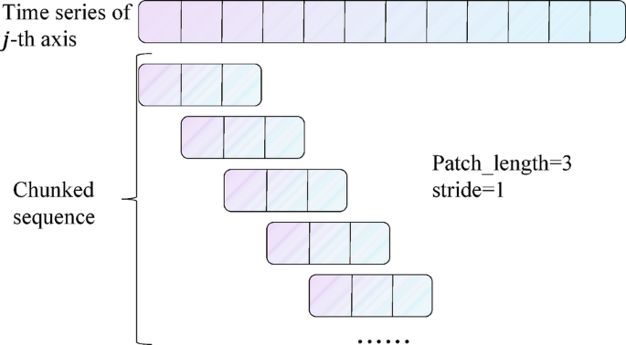
Example of patch operation.

All patches \(\:{\left\{{x}_{i}^{{\prime\:}}\left(j,p\right)\right\}}_{j,p=1}^{A,N}\) from every axis \(\:j\) are then independently mapped into a latent space of dimension \(\:D\) via a shared linear projection \(\:{\text{W}}_{\text{P}}\in\:{\mathbb{R}}^{D\times\:P}\), combined with positional embedding \(\:{\text{W}}_{\text{p}\text{o}\text{s}}\in\:{\mathbb{R}}^{D\times\:P}\) to preserve temporal order:

where \(\:{\stackrel{\sim}{x}}_{i}^{{\prime\:}}\left(j,\:\:p\right)\in\:{\mathbb{R}}^{\text{D}}\) represents the embedded patch token. These tokens are subsequently fed into a standard Transformer encoder for temporal modeling. The encoder employs multi-head self-attention to capture global dependencies across time steps. Each attention head operates in parallel, enabling efficient multidimensional feature interaction. The architecture further includes feed-forward networks with Gaussian Error Linear Unit (GELU) activation⁴³, residual connections around each sub-layer, and layer normalization for stable training and improved gradient flow. Notably, the same projection and Transformer weights are shared across all patches and all axes.

Recognizing that the features obtained above are extracted axis-independently and lack explicit modeling of inter-axis relationships, we introduce a depth-wise separable convolution module to facilitate cross-axis interaction and feature fusion. As illustrated in Fig. 1, let \(\:{f}_{i}^{{\prime\:}}\in\:{\mathbb{R}}^{A\times\:N\times\:D}\) denote the extracted feature for each input sample \(\:{x}_{i}^{{\prime\:}}\). We first average the features along the patch dimension for each axis, resulting in a condensed representation \(\:{\stackrel{\sim}{f}}_{i}^{{\prime\:}}\in\:{\mathbb{R}}^{A\times\:D}\). This feature is then processed via a depth-wise separable convolution block. Specifically, a channel-wise grouped 1D convolution with a kernel size of 3 (denoted as \(\:{Conv}_{1\times\:3}\)) is applied to each axis independently, capturing local cross-channel patterns. This is followed by a pointwise convolution (\(\:{Conv}_{1\times\:1}\)) to fuse information across all channels, producing an enhanced feature \(\:{\dot{f}}_{i}^{{\prime\:}}\in\:{\mathbb{R}}^{A\times\:{D}^{{\prime\:}}}\). The operation is formulated as:

Finally, the feature \(\:{\dot{f}}_{i}^{{\prime\:}}\) is flattened into a vector \(\:{z}_{i}^{{\prime\:}}\) of dimension of \(\:A\cdot{D}^{{\prime\:}}\), which is then passed through a fully connected layer for final classification.

Datasets

As shown in Table 1, the datasets used in this study comprise two distinct parts: a cross-species unlabeled dataset employed for model pre-training, and a species-specific labeled dataset used for fine-tuning. All data are sourced from publicly available open-source repositories. A detailed description of each dataset is provided below.

Cross-species unlabeled dataset

This dataset aggregates publicly accessible accelerometer data from cattle, sheep, and horses, totaling 576,897 unlabeled samples^12,16,44,45. Consistent with common practice in animal activity recognition², only triaxial accelerometer data are utilized, as this modality has been widely validated as both prevalent and effective for the task. Initially, the dataset was fully labeled across 13 categories of common animal behaviors. To simulate an unlabeled environment for model pre-training, we subsequently removed all labels.

Species-specific labeled dataset

This dataset comprises 42,943 annotated samples collected from five goats⁴⁶, encompassing five behavioral categories: standing (43.15%), grazing (35.35%), walking (20.19%), running (0.87%), and trotting (0.44%). A severe class imbalance is present, with an imbalance ratio of 98.05; the minority class, trotting, contains only 189 samples. This dataset is used for fine-tuning the pretrained model.

Implementation details

Data preprocessing

For the cross-species pre-training dataset, we applied a systematic preprocessing pipeline to ensure consistency across heterogeneous data sources. First, multiple publicly available datasets were cleaned and harmonized by standardizing their sampling rates. High-frequency recordings (e.g., 100 Hz) were down-sampled, while low-frequency data (e.g., 12.5 Hz) were up-sampled to 25 Hz via nonlinear interpolation. This rate was chosen based on previous studies indicating that 25 Hz provides a suitable balance between performance retention and computational efficiency². To maintain uniformity across datasets, only triaxial acceleration data (common to all sources) were retained. The signals were segmented using a 2-second sliding window and normalized through z-score standardization, resulting in a final tensor of dimensions 576,897 × 50 × 3. The same preprocessing steps, including 2-second window segmentation and z-score normalization, were applied to the species-specific labeled dataset, yielding a tensor of size 42,943 × 50 × 3.

Experimental setting

This study evaluates the effectiveness of the proposed method by comparing a classification model initialized with pretrained parameters (our method) against one with random initialization (baseline). The objective is to assess whether cross-species pre-training improves behavior recognition performance for the target species. We employ accuracy, precision, recall, F1-score, macro-average, and weighted-average as evaluation metrics to comprehensively assess model performance^47,48. The macro-average metric computes the arithmetic mean of per-class scores, giving equal weight to each class, whereas the weighted-average accounts for class imbalance by weighting each class’s score by its sample size.

Similar to previous studies^49,50,51, we employed the leave-one-subject-out validation method with three random repetitions to assess the generalization of the fine-tuned classification model. In each repetition, we randomly assigned one goat for testing, one for validation, and the remaining four for training, while ensuring that the testing and validation sets were derived from different goats across all three runs. The model was trained using a class-balanced cross-entropy loss function⁵², augmented with an L2 regularization term (weight decay = 0.01) to mitigate overfitting. Optimization was performed with the Adam optimizer at a learning rate of 1 × 10⁻⁴. Each training run consisted of 100 epochs with a batch size of 32. The model achieving the highest validation accuracy was saved and evaluated on the test set. An early stopping strategy with a patience of 10 epochs was applied during training. All experiments were implemented in PyTorch and executed on a single NVIDIA GeForce RTX 5090 GPU.